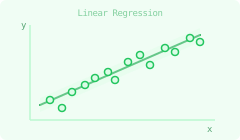
Statistics & Time Series

Overview

Statistical inference is the science of drawing conclusions about unknown parameters from data. This topic covers the foundational criteria for estimators, the two main estimation methods (MOM and MLE), confidence intervals, hypothesis testing, and linear regression. These tools appear directly in quant interviews involving data analysis, model validation, and quantitative research.

1. Estimator Properties

1.1 Bias, Variance, MSE

Definition

Let $\hat{\theta} = \hat{\theta}(X_1, \ldots, X_n)$ be an estimator of a parameter $\theta$ . The three fundamental quality criteria are:

\boxed{\text{Bias}(\hat{\theta}) = E[\hat{\theta}] - \theta}

\boxed{\text{Var}(\hat{\theta}) = E\!\left[(\hat{\theta} - E[\hat{\theta}])^2\right]}

\boxed{\text{MSE}(\hat{\theta}) = E\!\left[(\hat{\theta} - \theta)^2\right] = \text{Var}(\hat{\theta}) + \text{Bias}(\hat{\theta})^2}

An estimator is unbiased if $\text{Bias}(\hat{\theta}) = 0$ , i.e. $E[\hat{\theta}] = \theta$ .

Properties

MSE = Variance + Bias² $\quad$ (bias-variance decomposition)
Sample mean $\bar{X}_n$ is unbiased for $\mu$ : $E[\bar{X}_n] = \mu$

💡Tip

The bias-variance tradeoff is central to statistics and machine learning: reducing bias often increases variance and vice versa. In interviews, an unbiased estimator is not always preferable — a slightly biased estimator with much lower variance can have smaller MSE.

1.2 Consistency & Efficiency

Definition

An estimator $\hat{\theta}_n$ is consistent if:

\boxed{\hat{\theta}_n \xrightarrow{P} \theta \quad \text{as } n \to \infty}

Properties

Unbiased + $\text{Var}(\hat{\theta}_n) \to 0$ $\Rightarrow$ consistent
Consistent does not imply unbiased (and vice versa)
The MLE is consistent and asymptotically efficient under regularity conditions

1.3 Cramér-Rao Bound & Fisher Information

Definition— Fisher Information

For a model with density $f(x;\theta)$ , the Fisher information is:

\boxed{\mathcal{I}(\theta) = E\!\left[\left(\frac{\partial}{\partial\theta}\log f(X;\theta)\right)^2\right] = -E\!\left[\frac{\partial^2}{\partial\theta^2}\log f(X;\theta)\right]}

Theorem— Cramér-Rao Lower Bound

For any unbiased estimator $\hat{\theta}$ of $\theta$ :

\boxed{\text{Var}(\hat{\theta}) \geq \frac{1}{\mathcal{I}_n(\theta)} = \frac{1}{n\,\mathcal{I}(\theta)}}

💡Tip

Fisher information measures how much data tells you about $\theta$ . High Fisher information = sharper likelihood = more precise estimation. An estimator achieving the Cramér-Rao bound is called efficient — MLE achieves it asymptotically.

2. Estimation Methods

2.1 Method of Moments (MOM)

Definition

The method of moments estimates parameters by equating theoretical moments to empirical moments. For $k$ parameters $(\theta_1, \ldots, \theta_k)$ , solve:

Example

For $X \sim \Gamma(\alpha, \beta)$ : $E[X] = \alpha/\beta$ and $E[X^2] = \alpha(\alpha+1)/\beta^2$ . Setting and , solving gives and .

💡Tip

MOM is simple and always gives explicit formulas, but is generally less efficient than MLE. Use MOM when you need a quick closed-form estimator or as a starting point for MLE optimization.

2.2 Maximum Likelihood Estimation (MLE)

Definition

Given i.i.d. observations $X_1, \ldots, X_n \sim f(\cdot;\theta)$ , the likelihood and log-likelihood are:

Properties

Invariance: if $\hat{\theta}$ is the MLE of $\theta$ , then $g(\hat{\theta})$ is the MLE of $g(\theta)$

Example

For $X_i \sim \text{Exp}(\lambda)$ : $\ell(\lambda) = n\log\lambda - \lambda\sum X_i$ . Setting gives .

💡Tip

Always work with the log-likelihood $\ell(\theta)$ — products become sums, making differentiation tractable. For exponential family distributions, the MLE always has a clean closed form.

2.3 Asymptotic Properties of MLE

Theorem— Asymptotic Normality of MLE

Under regularity conditions, as $n \to \infty$ :

\boxed{\sqrt{n}(\hat{\theta}_{\text{MLE}} - \theta) \xrightarrow{d} \mathcal{N}\!\left(0,\, \frac{1}{\mathcal{I}(\theta)}\right)}

Remarque

This theorem says the MLE is asymptotically efficient — it achieves the Cramér-Rao bound in the limit. The asymptotic variance $1/(n\mathcal{I}(\theta))$ is the best possible variance for any unbiased estimator.

3. Confidence Intervals

3.1 Definition & Interpretation

Definition

A confidence interval (CI) at level $1-\alpha$ for parameter $\theta$ is a random interval $[L(X), U(X)]$ such that:

P (L (

Remarque

The CI is random, not $\theta$ . The correct interpretation: if we repeat the experiment many times, $(1-\alpha)\times 100\%$ of the constructed intervals will contain the true $\theta$ . It is wrong to say " $\theta$ has probability $1 -$ of being in the interval" — is fixed, not random.

3.2 CI for the Mean (known $\sigma$ )

Formula

For $X_1,\ldots,X_n$ i.i.d. with mean $\mu$ and known variance $\sigma^2$ , by the CLT:

3.3 CI for the Mean (unknown $\sigma$ )

Formula

For $X_1,\ldots,X_n$ i.i.d. $\mathcal{N}(\mu,\sigma^2)$ with , using :

Remarque

This uses the fact that $\dfrac{\bar{X}_n - \mu}{S/\sqrt{n}} \sim t(n-1)$ exactly under normality. As , and both formulas agree.

3.4 CI for a Proportion

Formula

For $X_1,\ldots,X_n$ i.i.d. Bernoulli $(p)$ with $\hat{p} = {\overset{ˉ}{X}}_{}$ :

💡Tip

The duality between CI and hypothesis tests: $\theta_0$ is rejected at level $\alpha$ by a two-sided test if and only if $\theta_0$ falls outside the $(1-\alpha)$ CI. This equivalence lets you read off test decisions directly from CIs.

4. Hypothesis Testing

4.1 Framework: $H_0$ , $H_1$ , Errors, $p$ -value

Definition

A hypothesis test decides between:

Null hypothesis $H_0$ : the default assumption
Alternative hypothesis $H_1$ : what we want to detect

The test statistic $T(X_1,\ldots,X_n)$ leads to rejection of when (rejection region).

Definition— Error Types & Power

\boxed{\alpha = P(\text{reject } H_0 \mid H_0 \text{ true}) \quad \text{(Type I error, significance level)}}

Definition—

p

-value

The $p$ -value is the probability, under $H_0$ , of observing a test statistic at least as extreme as the one observed:

\boxed{p\text{-value} = P_{H_0}(T \geq t_{\text{obs}})}

Remarque

The $p$ -value is not the probability that $H_0$ is true. It is the probability of the data (or more extreme) given $H_0$ is true. A small $p$ -value means the data is unlikely under , not that is unlikely.

4.2 Common Tests

Properties— Standard Tests

Test	$H_0$	Statistic	Distribution under $H_0$
$z$ -test	$μ =$ ( known)

💡Tip

Memory rule: use $z$ when $\sigma$ is known, $t$ when $\sigma$ is unknown. The $\chi^2$ test for variance and the $F$ -test for equality of variances both require normality — they are sensitive to this assumption.

4.3 Neyman-Pearson Lemma

Theorem— Neyman-Pearson Lemma

For testing $H_0: \theta = \theta_0$ vs $H_1: \theta = \theta_1$ (simple hypotheses), the test at level rejects when:

Remarque

The likelihood ratio test is optimal in the sense of maximizing power for a given significance level. For composite hypotheses, the generalized likelihood ratio test uses $\Lambda = \sup_{\theta \in H_1} L(\theta) / \sup_{\theta \in H_0} L(\theta)$ and under (Wilks' theorem).

5. Linear Regression

5.1 Model & Assumptions

Definition

The linear regression model assumes:

\boxed{\mathbf{y} = X\boldsymbol{\beta} + \boldsymbol{\varepsilon}, \quad \boldsymbol{\varepsilon} \sim \mathcal{N}(\mathbf{0}, \sigma^2 I_n)}

Properties— Gauss-Markov Assumptions

L1: $E[\boldsymbol{\varepsilon}] = \mathbf{0}$ $\quad$ (zero mean errors)
L2: $\text{Cov}(\boldsymbol{\varepsilon}) = \sigma^2 I_n$ (homoscedasticity, no correlation)

5.2 OLS Estimator

Theorem— OLS Estimator

The ordinary least squares estimator minimizes $\|\mathbf{y} - X\boldsymbol{\beta}\|^2$ and is given by:

\boxed{\hat{\boldsymbol{\beta}} = (X^TX)^{-1}X^T\mathbf{y}}

Properties

$E[\hat{\boldsymbol{\beta}}] = \boldsymbol{\beta}$ $\quad$ (unbiasedness under L1--L3)
$\text{Cov}(\hat{\boldsymbol{\beta}}) = \sigma^2(X^TX)^{-1}$

5.3 Gauss-Markov Theorem

Theorem— Gauss-Markov

Under assumptions L1--L3, the OLS estimator $\hat{\boldsymbol{\beta}}$ is the Best Linear Unbiased Estimator (BLUE): among all linear unbiased estimators $\tilde{\boldsymbol{\beta}} = C\mathbf{y}$ ,

Remarque

Gauss-Markov does not require normality — only L1--L3. Adding normality (L4) gives exact $t$ and $F$ distributions for inference. Without normality, the CLT provides approximate inference for large $n$ .

5.4 Goodness of Fit ( $R^2$ )

Definition

The coefficient of determination $R^2$ measures the proportion of variance in $\mathbf{y}$ explained by the model:

\boxed{R^2 = 1 - \frac{\text{SS}_{\text{res}}}{\text{SS}_{\text{tot}}} = 1 - \frac{\|\mathbf{y}-\hat{\mathbf{y}}\|^2}{\|\mathbf{y}-\bar{y}\mathbf{1}\|^2} \in [0,1]}

Properties

$R^2 = 0$ : model explains nothing; $R^2 = 1$ : perfect fit
$R^2$ increases with every added predictor — use to penalize complexity:

💡Tip

A high $R^2$ does not imply a good model — it can be inflated by irrelevant predictors (use adjusted $R^2$ ), by outliers, or by spurious correlations. Always check residual plots alongside $R^2$ .

6. Quick Reference

Estimator Criteria

Criterion	Definition
Unbiased	$E[\hat{\theta}] = \theta$
MSE	$\text{Var}(\hat{\theta}) + \text{Bias}^2$

Confidence Intervals

Parameter	CI
$\mu$ ( $\sigma$ known)	$\bar{X} \pm z_{\alpha/2}\,\sigma/\sqrt{n}$

Regression Formulas

Concept	Formula
OLS estimator	$\hat{\boldsymbol{\beta}} = (X^TX)^{-1}X^T\mathbf{y}$

Statistics & Time Series

1. Estimator Properties

1.1 Bias, Variance, MSE

1.2 Consistency & Efficiency

1.3 Cramér-Rao Bound & Fisher Information

2. Estimation Methods

2.1 Method of Moments (MOM)

2.2 Maximum Likelihood Estimation (MLE)

2.3 Asymptotic Properties of MLE

3. Confidence Intervals

3.1 Definition & Interpretation

3.2 CI for the Mean (known σ\sigmaσ)

3.3 CI for the Mean (unknown σ\sigmaσ)

3.4 CI for a Proportion

4. Hypothesis Testing

4.1 Framework: H0H_0H0​, H1H_1H1​, Errors, ppp-value

4.2 Common Tests

4.3 Neyman-Pearson Lemma

5. Linear Regression

5.1 Model & Assumptions

5.2 OLS Estimator

5.3 Gauss-Markov Theorem

5.4 Goodness of Fit (R2R^2R2)

6. Quick Reference

Estimator Criteria

Confidence Intervals

Regression Formulas

3.2 CI for the Mean (known $\sigma$ )

3.3 CI for the Mean (unknown $\sigma$ )

4.1 Framework: $H_0$ , $H_1$ , Errors, $p$ -value

5.4 Goodness of Fit ( $R^2$ )